Summary
cumulativeHisto([<timeWindow>,] [<bucketName>,] <tsExpression>
   [,metrics|sources|sourceTags|pointTags|<pointTagKey>] )
Converts a cumulative histogram coming from Prometheus, Telegraf, or other source to an ordinary histogram in Operations for Applications histogram format. Users can then manipulate the histogram with Operations for Applications histogram query functions.
_bucket metric. The _count and _sum metrics won’t return results. Parameters
| Parameter | Description |
|---|---|
| timeWindow | Amount of time in the moving time window. You can specify a time measurement based on the clock or calendar (1s, 1m, 1h, 1d, 1w), the window length (1vw) of the chart, or the bucket size (1bw) of the chart. Defaults to 1m. |
| bucketName | Optional string that describes the bucket. Default is le, that is, less than or equal. If your source histogram uses a different tag key to specify the buckets, specify that tag key here. |
| tsExpression | Cumulative histogram that we'll convert to an ordinary histogram. |
| metrics|sources|sourceTags|pointTags|<pointTagKey> | Optional group by parameter for organizing the time series into subgroups and then returning each histogram subgroup.
Use one or more parameters to group by metric names, source names, source tag names, point tag names, values for a particular point tag key, or any combination of these items. Specify point tag keys by name. |
Description
This function is useful if you want to analyze data that are already in a cumulative histogram format.
This function works only with data that include a parameter such as le for defining which part of the cumulative histogram you want to display. Data that are imported from Prometheus always include such a parameter.
When a chart displays the result of this function, it shows the median by default. You can use percentile() to change that and, for example, show the 90% percentile.
Ordinary and Cumulative Histograms
Operations for Applications histogram distributions are ordinary histograms. In contrast, some other tools, such as Prometheus and Telegraf, use cumulative histograms.
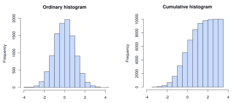
(image credit: Wikipedia)
If your data source emits cumulative histograms, you can use this function to visualize your histogram data in Operations for Applications dashboards and charts.
How to Map Prometheus Queries to Operations for Applications Queries
When you use Prometheus, you run queries like this:
histogram_quantile(0.90, sum(rate(req_latency_bucket[5m])) by (le))
This query displays the 90th quantile of a cumulative histogram that corresponds to the req_latency_bucket metric. The le parameter means less than or equal.
The corresponding Operations for Applications query looks like this:
percentile(90, cumulativeHisto(sum(rate(ts(req_latency_bucket)), le)))
Here, we are creating a T-digest and adding sampling points based on the range and the count of the bucket.
Grouping
Similar to aggregation functions for metrics, cumulativeHisto() returns a single distribution per specified time window. To get separate distributions for groups that share common characteristics, you can include a group by parameter, as for many ts() queries. For example, use cumulativeHisto(1m, <expression>, sources) to group by sources.
The function returns a separate series of results for each group.
zone and ZONE, when you use an aggregation function and apply grouping, we consider zone and ZONE as separate tags. Interpolation
The cumulativeHisto() function itself doesn’t perform interpolation because that doesn’t make sense for a histogram. But when you apply percentile(), we do perform interpolation.
See Standard Versus Raw Aggregation Functions.
Using taggify() with Prometheus Metrics from Telegraf
When you use Telegraf to collect Prometheus histogram metrics, the metrics include the bucket bounds as part of the metric names. For example:
source.source_http_requests_latency_including_all_seconds.2.5
source.source_http_requests_latency_including_all_seconds.5.0
source.source_http_requests_latency_including_all_seconds.10.0
If you want to use these metrics with WQL and show them in our dashboards and charts:
- Extract the buckets as tags using
taggify() - Apply
cumulativeHisto()
For example:
-
You start with data metrics like this:
data:
mavg(5m, rate(ts(“metric1_seconds.*" and not “metric1_seconds.count" and not “metric1_seconds.sum" ))) -
You use
taggify()to extract the bucket information.taggify:
sum(taggify(${data}, metric, le, "^metric1_seconds.(.*)$", "$1"), le) -
Now you can apply
cumulativeHistoand other functions to the result.target_data:
percentile(95, cumulativeHisto(${tagged}))
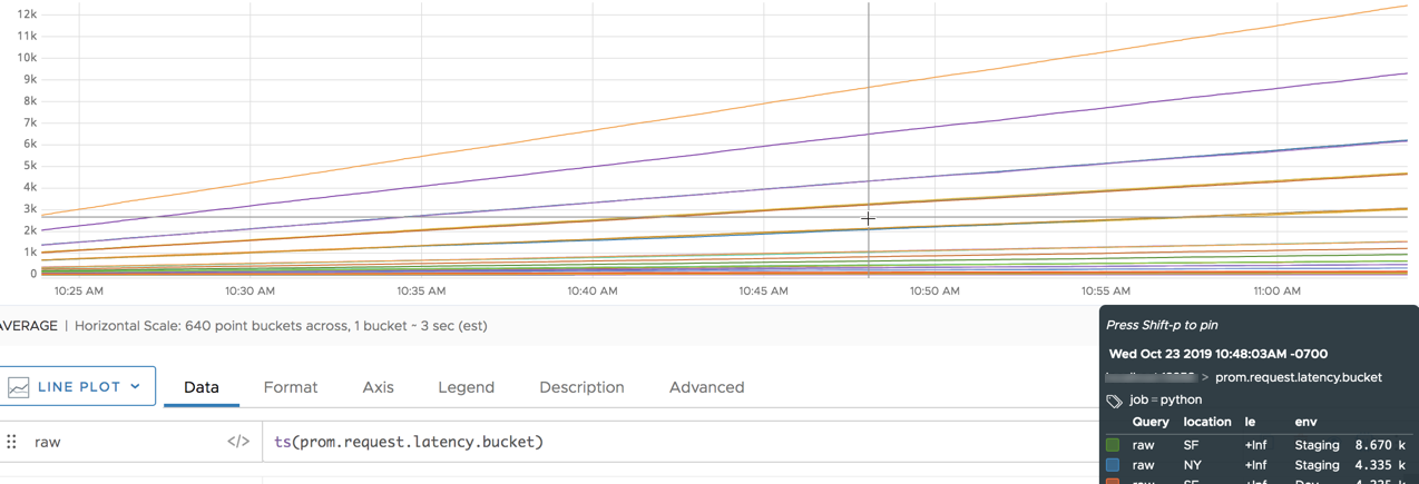
Example
The following example starts with a cumulative histogram in Prometheus format. We can show only histogram values that are less than or equal to 60 using the le tag. You can see the le tag in the legend.
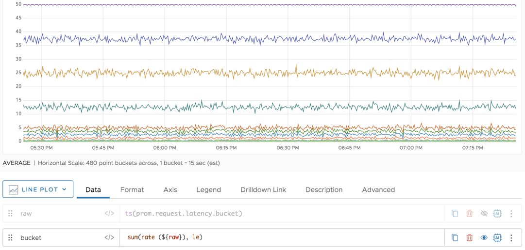
We can then manipulate the cumulative histogram. First, we use sum(rate()) to return the per-second rate of each time series.
See Also
- The cumulativePercentile function doc page that explains how to calculate the cumulative percentile without the need to convert the cumulative Prometheus histogram to an Operations for Applications ordinary histogram.
- This blog post discusses the Prometheus integration in some detail.
- The How to Make Prometheus Monitoring Enterprise Ready blog post explores how using Prometheus for metrics collection and Operations for Applications for data storage and visualization can give you the best of both worlds.
- Our histogram doc page gives background information about Operations for Applications histograms.
Caveats
This function is meant for cumulative histograms, like those that come from Prometheus or Telegraf. It’s not useful for ordinary histogram distributions.